Background

Percolation theory is the study of the behaviour of the random subgraphs obtained when adding edges to a lattice with a given probability $p$. More precisely, what we have just described is bond percolation - in the alternate model of site percolation nodes are occupied with a given probability, with edges then implicitly drawn to all neighbouring occupied nodes. Unless otherwise specified, we will always be referring to bond percolation from now on.

We are typically interested in studying the behaviour of the connected components of the percolation as $p$ varies. For the case of infinite lattices, we ask the question: Are there infinite clusters? If so, how many, and how does this depend on $p$?

Obviously, for $p=0$, every cluster has size 1, and for $p=1$, there is one single infinite cluster. By Kolmogorov’s zero–one law, the probability of there being an infinite cluster for a given $p$ is either 0 or 1. It is not hard to show that this is an increasing function of $p$. We therefore obtain that there must be a critical value $p_c$ such that for every $p<p_c$, there are no infinite clusters, and for $p>p_c$ there is always an infinite cluster.

Simulation

Without referring to any prior research in the field, two obvious ways of simulating this behaviour stood out to me.

The first would be a way of simulating the growth of a single cluster: Starting at a given point, add all of the neighbours (along a valid edge in the lattice) to a queue each with probability $p$, then add the point to the visited set. Continue the algorithm by popping a neighbour off the queue, adding all unvisited neighbours to the back of the queue with probablity $p$, then adding the current point to the visited set and so on. If the cluster was finite, the algorithm would terminate when the queue of neighbours was empty.

With this algorithm we obtain $O(N)$ runtime and memory usage.

The second would be to use a disjoint set forest data structure: We iterate over every possible edge in the lattice and merge the two clusters at each point with probability $p$.

With this method (using union by size and path halving) we obtain $O(N)$ memory usage and $O(N\alpha(N))$ runtime (where $\alpha$ is the inverse Ackermann function, which can be considered essentially constant for our purposes).

The second method has the obvious advantage of simulating the entire system, not just a single cluster, therefore we shall choose the latter as both offer comparable performance. And you can generate pretty pictures like this!

Considerations

We choose union by size, rather than union by rank for the obvious reason of keeping track of the size of each cluster.

Since maintaining a hash map of coordinates to their given element in the forest is relatively slow and space inefficient, we choose instead to index coordinates to a flattened vector of elements of fixed size to represent the forest. This offers another advantage in the following: In a typical disjoint set forest implementation, we store the value of the node, the value of the parent and the size (or rank) for each element in the forest. This would, for example, use 28 bytes per node if using 32 bit integers for 3D coordinates and size. Instead, we only store one size_t for the index of the parent node, and one 32 bit integer for the size of the cluster - the index of the current node can be calculated from its address: Thus we use only 12 bytes per node (using tight struct packing).

Our disjoint set forest implementation requires simply implementing two functions to be used for any lattice: One function mapping coordinates to a unique index, and the other its inverse.

Parallelising the algorithm is straightforwad - we simply slice up the domain and simulate the percolation in each slice, before merging together.

Pseudorandom numbers are generated using a permuted congruential generator (PCG) with 128 bits of internal state and 64 bit output, based on their speed and strong performance on statistical tests such as TestU01.

Analysis of results

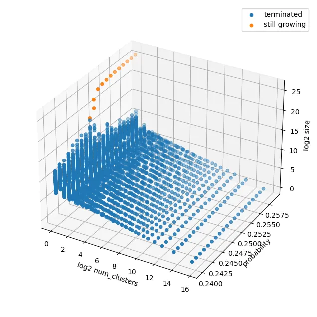
We begin with a simple plot to give us a starting point and validate that our simulation is giving sensible results. We would expect that significantly below the critical value, all of the percolation clusters in our simulation would terminate, whilst significantly above the critical value there would be one single cluster which dominates, and does not terminate. A simple plot of log cluster size against log number of clusters over a range of probabilities shows this clearly.

Let $n_s(p)$ be the average number of clusters per lattice point of size $s$ for a given probability $p$. According to standard scaling theory (e.g. [MM]) we have that

where $\tau$ is the fisher exponent, $\Omega$ accounts for the leading errors due to the finite size of our lattices, $z=(p-p_c)s^{\sigma}$ for some constant $\sigma$ and $f_0, f_1...$ are analytic in a neighbourhood of zero. Taking the taylor expansion of the $f_i$ we obtain

Taking logs, pulling out a constant factor and taking the Taylor expansion of the $f_i$, we obtain

in a neighbourhood of $p_c$. Thus (aside from the effects of $\Omega$) we expect the critical value to occur when we have a log-linear relationship between $n_s$ and $s$. This aligns well with our initial sanity-check plot.

It will be convenient for our simulations to sample individual points from our lattice, rather than counting clusters. So we instead consider the probability $P(s)$ that a given point lives in a cluster of size $s$, which is simply $sn_s$.

One obstacle we must overcome if we wish to make accurate predictions is the fact that our simulations must always be finite. In order to remove boundary effects, it is convenient to consider the cumulative distribution $Q(s) = \sum_{t=s}^{\infty}P(t)$. This way, we can simply collect up all the terms affected by the boundary into the final bin. Approximating this as an integral, we obtain

(note that we have absorbed some constant factors into the $c_i$ when evaluating the integral) and so

Thus to obtain accurate estimates for $p_c$ (and $\tau$) it remains to generate as much data as possible on the relationship between $n_s$ and $s$, whilst minimising the effects of finite lattice sizes.

We shall therefore sample the size of the parent cluster for all of the points from a smaller central cube of side length $L'$ from our lattice of side length $L$, and sum up our results over a large number of runs.

First, let us zoom in a bit from out initial sanity check plot and obtain a sensible starting point to look for $p_c$.

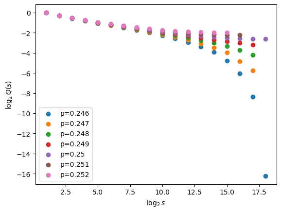
From this plot we can clearly see that $p_c$ should be somewhere in the region of 0.249, as we are close to linear here as we would expect - probably slightly below this value as $p=0.248$ is somewhat closer to linear than $p=0.25$.

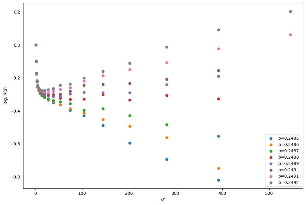
Upon running further simulations (200 runs for lattice size $L=512$, sampling from a central cube of side length 64, for $p$ in the range 0.2485-0.2492) we obtain the following fit (using least squares regression)

p_c   = 0.24886253574635508       std dev = 1.493182835296289e-05
tau   = 2.186571141359527         std dev = 0.0018298030787328374
omega = 0.5703627813634904        std dev = 0.04426674919925896
sigma = 0.47844360077149967       std dev = 0.015774739005157655
a_0   = -0.12876643226983475      std dev = 0.020368144930110438
a_1   = 3.3707734376292744        std dev = 0.5968482998817858
a_2   = 0.4695729949018457        std dev = 0.015109919403050643
a_3   = -5.138443437247822        std dev = 9.33286680486532

We can use these initial estimates for $p_c$, $\tau$, $\Omega$ and $\sigma$ as follows.

In order to estimate for $p_c$ as accurately as possible, it is helpful to now remove the main term from (1). With this in mind, let $R(s)=s^{\tau-2}Q(s)$. Then

Plotting this we obtain

Differentiating with respect to $s^{\sigma}$ (as used in [LZ]) gives

And so when close to $p_c$ for large $s$, we should obtain a linear relationship between $\frac{\partial\log R(s)}{\partial s^{\sigma}}$ and $p$, with the $p$-intercept giving $p_c$.

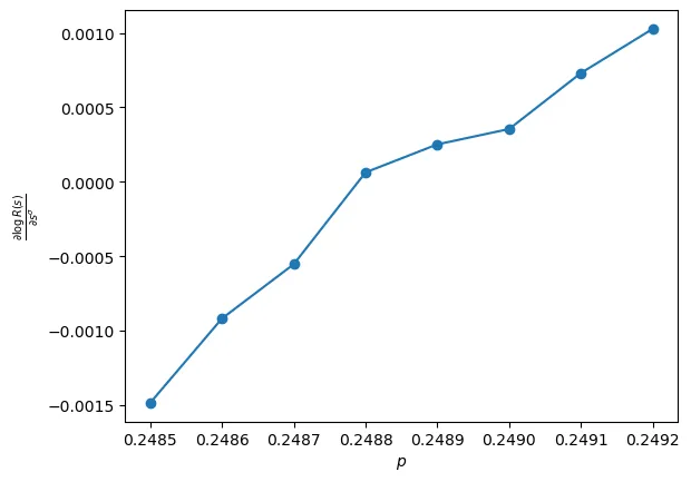
From this it looks like the critical value must be around the $p=0.2488$ mark. The (approximate) linearity of the plot gives us some confidence that our model in (2) is correct. I will return to this in the near future with slightly more powerful hardware to obtain a more precise estimate. Note that all of the above simulations have been run on WSL running on my 6 year old budget laptop (with 0% battery health) with only 4GB of available RAM and 4 mediocre CPU cores… So it should be possible to obtain much better results with some actual compute and memory.

For access to the source code used in this article, as well as the data used in the above plots, please see my github repo.

Bibliography

[MM] S. Mertens and C. Moore, Phys. Rev. E 98, 022120 (2018)

[LZ] C.D. Lorenz and R.M. Ziff, Phys. Rev. E 57, 230 (1998)